OpenPose and 3D Reconstruction – Part 3: 3D Reconstruction

This is Part 3 of the series on capturing human motion with OpenPose and reconstructing it in 3D. In Part 1 we set up OpenPose and got 2D keypoints; in Part 2 we calibrated the cameras and computed projection matrices. Now we reach the payoff: turning 2D keypoints from many cameras into 3D. This post assumes you’ve watched Parts 1 and 2.

Three topics:

3D reconstruction with the Direct Linear Transform (DLT / triangulation)
Filtering the reconstructed data
Optimization by minimizing reprojection error

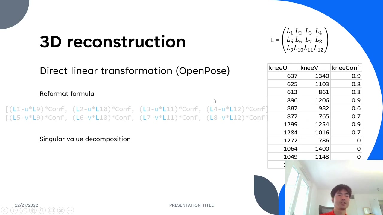
1. Triangulation with the Direct Linear Transform (DLT)

The core idea is to find where multiple projection lines cross. From a single camera, a 2D keypoint plus that camera’s projection matrix defines a ray into 3D space — but you can’t know where along the ray the real point sits. Add a second camera at a different angle, and the two rays intersect at the 3D point. That’s triangulation.

Two cameras with image planes and projection rays meeting at a 3D point — Two views triangulate a 3D point. Diagram credit: O. H. Maghsoudi (2019), as shown in the video.

In practice the rays rarely meet exactly — there’s a small gap — so you estimate the midpoint between them. Mathematically: 2D = intrinsics × extrinsics × 3D, where projection matrix = intrinsics × extrinsics. You rearrange this into the DLT equations, stack two rows (for the x and y image coordinates) per camera across all views into one large matrix, and solve with Singular Value Decomposition (SVD). The solution is the 3D point.

2. Weighting by OpenPose confidence

OpenPose outputs more than 2D coordinates — it gives a confidence score for each keypoint. You can fold that confidence into the DLT by multiplying each camera’s equations by its confidence. The effect: the estimated midpoint shifts toward the rays from high-confidence cameras and away from uncertain ones, which improves accuracy. Everything else (the SVD) stays the same.

Confidence-weighted DLT: the L projection matrix, the reformatted equations multiplied by confidence, and a table of kneeU, kneeV, kneeConf values — Each DLT row is multiplied by the keypoint’s confidence. Note the sample table: some keypoints have confidence 0 (undetected).

The Python is compact: build the matrix from each camera’s projection-matrix parameters and undistorted (u, v) points, then take the SVD; the 3D coordinates come from the last row of Vh, normalized by its last element.

Python DLT reconstruction: building matrix M from projection params and 2D points, then np.linalg.svd and xyz = Vh[-1,0:-1] / Vh[-1,-1] — The DLT reconstruction: stack per-camera rows, SVD, then read the 3D point from the last singular vector.

Getting the data out of OpenPose (JSON) and tracking a person

OpenPose writes one JSON file per frame. In MATLAB you read the file, use jsondecode to get a struct, and pull out the keypoints with dot-notation — easy to automate. The catch: OpenPose detects multiple people but does not track them across frames, so a person’s ID can switch or disappear between frames.

To follow the right person, the tutorial uses a simple tracker: on the first frame you select the subject; on each next frame, compare the previous pose to every detected person and keep the one with the lowest error. If the best match still exceeds ~100 px, it stops and asks you to re-select the subject. It’s semi-automatic, but it favors accuracy. After extraction, separate the confidence from the x/y coordinates, fill any missing (zero) keypoints (linear interpolation works well enough), and smooth.

3. Filtering: choosing the cutoff with residual analysis

To smooth the data a Butterworth filter is common, but the hard question is always: what cutoff frequency? Residual analysis answers it objectively. Sweep a range of cutoffs (e.g. 1–10 Hz in 0.1 steps), and at each one compute the residual — the RMS error between the original and filtered signal — then plot residual vs. cutoff.

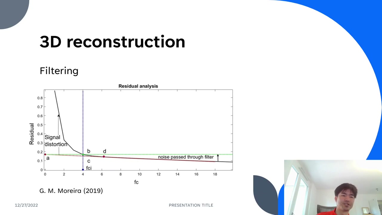
Residual analysis plot: residual vs cutoff frequency, with signal distortion at low cutoff and noise passed through at high cutoff, and the optimal cutoff fci — Residual analysis: extend the flat (noise) tail to the y-axis, draw a horizontal line, and its crossing gives the optimal cutoff. Diagram credit: G. M. Moreira (2019), as shown in the video.

At a very low cutoff you filter out real signal (large residual, “signal distortion”); at a high cutoff you pass the noise through (residual flattens toward the noise floor). Take the flat tail, extend its slope to the y-axis, draw a horizontal line from there, and where it crosses the curve gives the optimal cutoff frequency — the sweet spot that removes noise without eating the signal. Then filter with that cutoff.

The author is candid that where in the pipeline to filter — right after OpenPose, after 3D reconstruction, or elsewhere — is still an open question worth experimenting with.

4. Optimization: minimizing reprojection error

Finally, an optional refinement. Using a least-squares optimizer (SciPy’s least_squares) you refine the reconstructed 3D by minimizing the reprojection error: take the reconstructed 3D point, project it back to 2D through each camera’s projection matrix, and compare to the original OpenPose 2D point. The gap is the error; minimize it across all cameras. You can again weight each camera’s error by its OpenPose confidence.

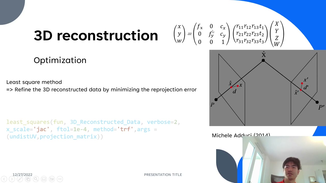
Optimization slide: least_squares call and a reprojection-error diagram showing observed vs reprojected 2D points — Refining 3D by minimizing reprojection error with SciPy least_squares. Reprojection diagram credit: Michele Adduci (2014), as shown in the video.

An honest caveat from the video: this assumes the OpenPose 2D points are the “truth” to minimize against — but they are themselves estimates. If the reference is imperfect, minimizing error against it may or may not help. In the author’s experience it improves some cases and hurts others. If you know a principled answer here, he’d genuinely like to hear it in the comments.

Coming next

With 3D motion reconstructed, the final parts of the series move into biomechanics: kinematic and kinetic simulation. Subscribe on YouTube so you don’t miss them.

About the author

Takashi Fukushima — research & development across Sports & Exercise Science, Human Pose Estimation, Computer Vision, and XR.

YouTube (subscribe): Takashi Fukushima｜Sports Science & Pose Estimation
Research (ORCID): orcid.org/0000-0002-7318-3384
Website: takashifukushima.com
Contact: Get in touch