This is the hands-on companion to The Biomechanics of a Soccer Kick. There we broke a kick into phases; here we do the actual analysis in MATLAB — taking the raw OpenPose JSON output and turning it into joint angles, clean filtered signals, phase timings, and a results table.
1. Import the OpenPose JSON
OpenPose writes one JSON file per frame. List them with dir, then loop through: read each file with fileread, parse it with jsondecode, and pull out data{i}.people(1).pose_keypoints_2d. That vector is laid out as X, Y, confidence for each of the 25 BODY_25 joints, so you split it into three matrices — X = P(1:3:end), Y = P(2:3:end), and Conf = P(3:3:end) — giving 25 joints × the number of frames (64 here).
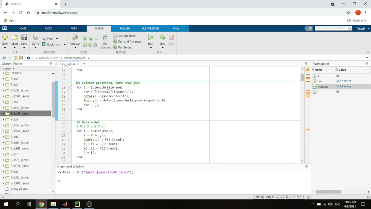
The joint order is fixed by OpenPose (search “OpenPose BODY_25” for the map), so once you know it you know which row is which joint.
2. Compute the joint angles
A joint angle is the angle between two limb segments. For the knee, take the vector from knee to ankle and the vector from knee to hip, and use the two-argument inverse tangent for a robust result: atan2d(|det([v1; v2])|, dot(v1, v2)). The determinant gives the “opposite” (cross-product magnitude) and the dot product the “adjacent”. Then subtract from 180° to get the anatomical angle.
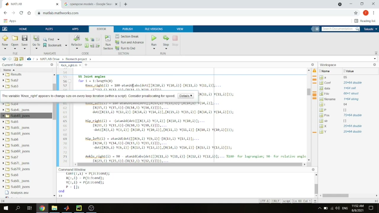
A few joint-specific tweaks:
- Knee:
180 - atan2d(...). A knee won’t realistically pass 180°. - Hip: don’t subtract 180 — the hip can go beyond it. Use the sign to separate back swing (negative) from forward swing (positive); for the right hip you also flip the sign (mirror side) and negate the dot product so the signs come out right.
- Ankle:
90 - atan2d(...), because a neutral standing ankle is about 90°.
3. Filter the data (choose the cutoff with a power spectrum)
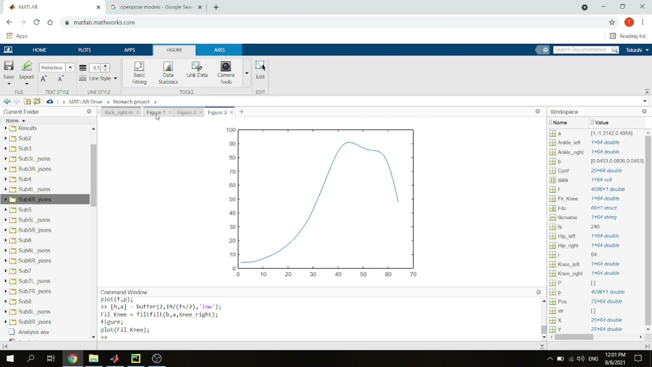
The raw angle traces are noisy, so smooth them with a Butterworth low-pass filter. The only real decision is the cutoff frequency — and you can pick it objectively from the power spectrum. With the frame rate as the sampling frequency (fs = 240), run pspectrum(angle, fs) and plot power vs. frequency: the real signal sits at low frequencies and the power falls off into a noise floor. Here that transition is around 19 Hz.
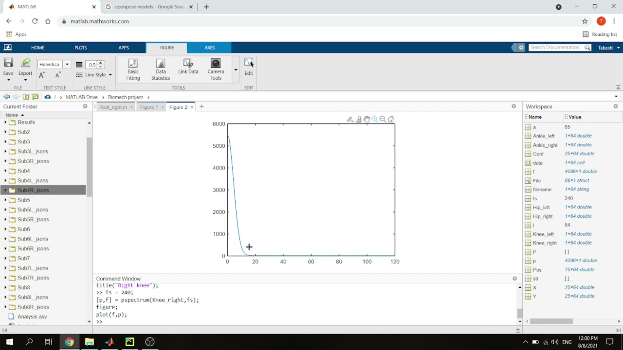
Then build the filter with [b,a] = butter(2, 19/(fs/2), 'low') and apply it with zero-phase filtfilt(b, a, angle). The result is a clean, smooth trace.
4. Angular velocity, phases, and landing
From the smoothed angles you compute angular velocities (and their maxima), then locate the phases from the same kinematics used in the biomechanics article. The maximum hip angle marks the end of the back swing; the maximum knee angle marks leg cocking and leg acceleration. Each phase is expressed as a percentage of the movement (its frame index divided by the total, times 100).
The one event that needs care is landing of the support foot. You can find it automatically — the frame where the ankle’s vertical position is lowest — or simply scrub the image frames and read it off by eye (here, about frame 45). The supporting-leg phases (shock absorption, energy transfer) then follow from its knee kinematics.
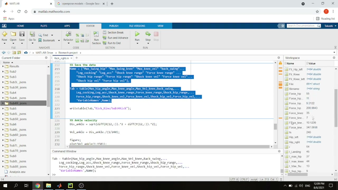
5. Collect the results into a table
Finally, gather everything into a named MATLAB table — 14 variables such as maximum swing-leg hip angle (51°), maximum knee angle (90°), maximum knee angular velocity, and the shock-absorption and energy-transfer ranges and velocities for hip and knee. writetable saves it to CSV so you can compare subjects or trials.
Takeaway
That’s a complete, reproducible pipeline: OpenPose keypoints in, joint angles and phase metrics out — all in a few dozen lines of MATLAB. The same logic ports cleanly to Python if you prefer free tools. Pair it with the biomechanics breakdown and you have both the “what” and the “how” of markerless kick analysis.
About the author
Takashi Fukushima — research & development across Sports & Exercise Science, Human Pose Estimation, Computer Vision, and XR.
- YouTube (subscribe): Takashi Fukushima|Sports Science & Pose Estimation
- Research (ORCID): orcid.org/0000-0002-7318-3384
- Website: takashifukushima.com
- Contact: Get in touch