This is the final part of the series on capturing human motion with OpenPose and reconstructing it in 3D. We set up OpenPose (Part 1), calibrated cameras (Part 2), reconstructed 3D motion (Part 3), and ran kinematics in OpenSim (Part 4). Now we go one level deeper into biomechanics: kinetic (dynamic) simulation — estimating muscle activations and ground reaction forces.
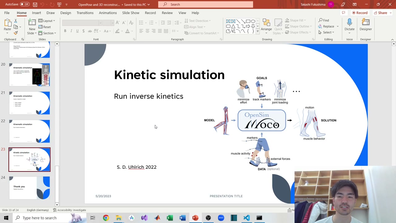
Under the hood, OpenCap uses OpenSim Moco (an optimal-control library) together with automatic differentiation. It fuses the scaled musculoskeletal model with the kinematics from Part 4 and solves for how the muscles must have worked — and what ground reaction forces were involved — to produce that motion.
Setting up the dynamic simulation
The relevant Python lives in OpenCap’s UtilsDynamicSimulations and its automatic-differentiation code (OpenSimAD). Clone the OpenCap repository, append those paths, and import the two functions you need. Then point them at your scaled model and the motion/kinematics file from Part 4.
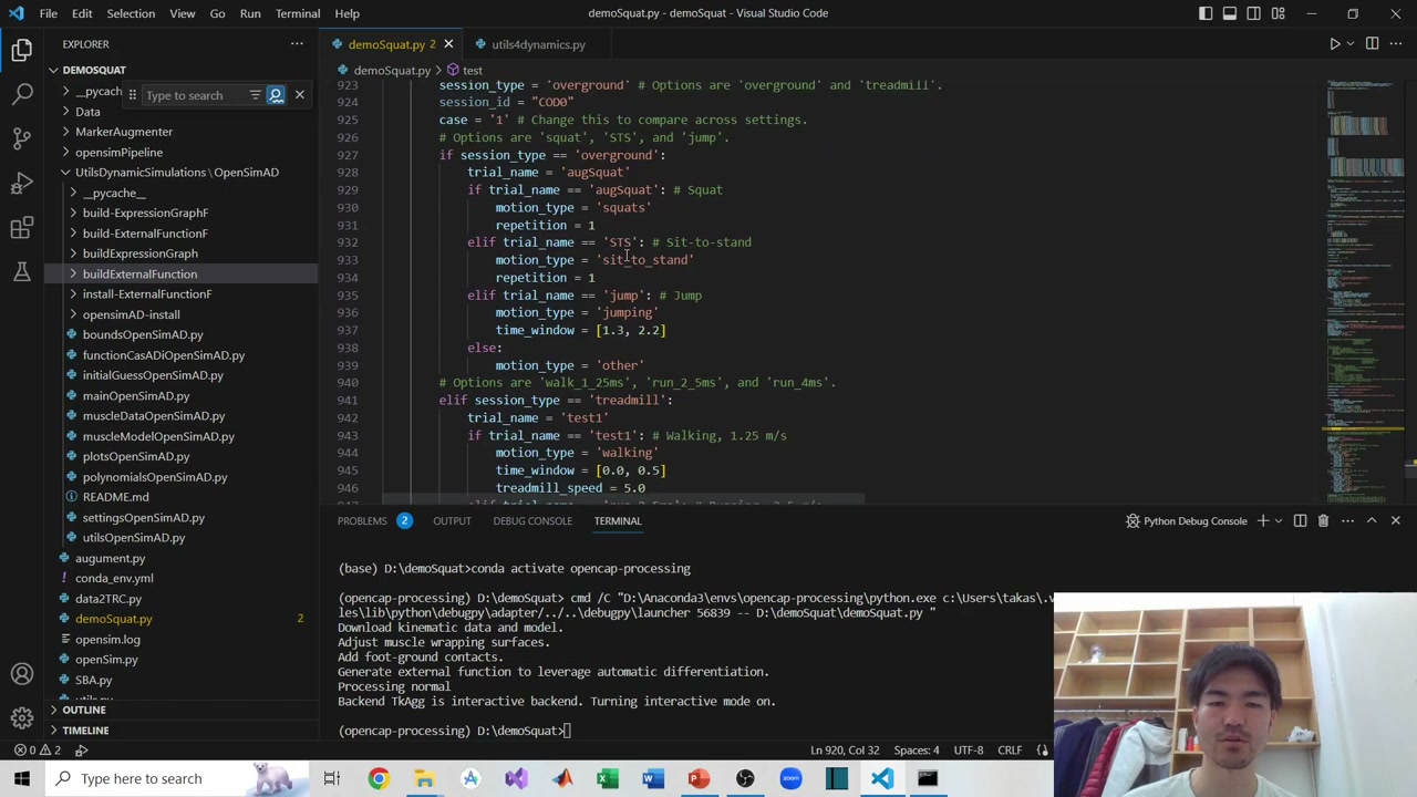
OpenCap exposes a few configurations: whether the motion is overground or on a treadmill, and the motion type (squat, sit-to-stand, jump, walking, running…). Here it’s a squat, so motion_type = 'squats'. Make sure the trial name matches the motion file name. Then plug the variables in and run the tracking function.
Watch the time window. Repetitive motions (squat, sit-to-stand) are handled per repetition. For continuous motions (walking, running) you set a time window — but it must be within about 2 seconds. Longer windows tend to fail to converge (too many iterations), so keep them short.
When you run it, the pipeline takes a while: it downloads/adjusts the model, adds muscle wrapping surfaces and foot-ground contacts, generates an external function for automatic differentiation, computes the Jacobian, and then solves. When it finishes, the kinetic data is ready.
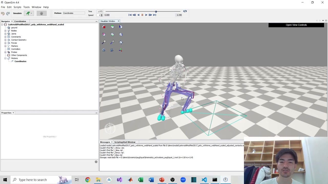
Muscle activations
The results land in an auto-created Dynamics folder (with a subfolder named after your motion). Open the scaled model in the OpenSim GUI and load the activations motion file. As it plays, each muscle is colored by its activation — you can see which muscles are working through the movement.
Ground reaction forces
You can also visualize the ground reaction force (GRF). Use “associate motion data” to load the resultant GRF (combined across x, y, z) — it appears as an arrow, pointing upward as you’d expect for a squat. If you prefer, you can load the GRF components separately.
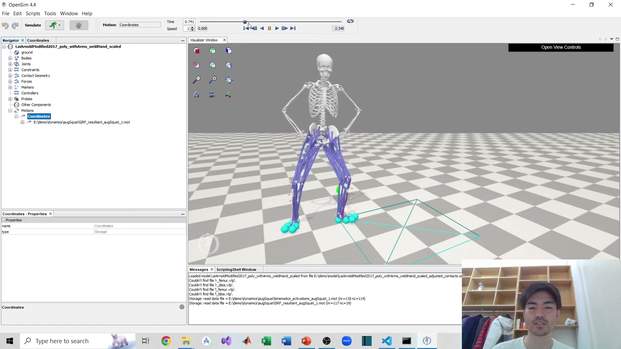
As in the previous parts, the squat is slightly distorted because of the imperfect calibration — but the result is genuinely usable. And that’s the point: starting from nothing but video and OpenPose (or any pose estimator), you can now estimate full dynamics thanks to OpenCap and OpenSim. It’s a real glimpse of the potential of markerless motion capture.
The full series
- Part 1 — OpenPose setup
- Part 2 — Camera calibration
- Part 3 — 3D reconstruction
- Part 4 — Kinematic simulation
- Part 5 — Kinetic simulation (this post)
Thanks for following the whole series. Questions are welcome in the YouTube comments or via the contact form.
About the author
Takashi Fukushima — research & development across Sports & Exercise Science, Human Pose Estimation, Computer Vision, and XR.
- YouTube (subscribe): Takashi Fukushima|Sports Science & Pose Estimation
- Research (ORCID): orcid.org/0000-0002-7318-3384
- Website: takashifukushima.com
- Contact: Get in touch