OpenPose and 3D Reconstruction – Part 4: Kinematic Simulation

This is Part 4 of the series on capturing human motion with OpenPose and reconstructing it in 3D. So far we set up OpenPose (Part 1), calibrated the cameras (Part 2), and reconstructed 3D motion (Part 3). Now we drive a biomechanical model with that motion: kinematic simulation in OpenSim.

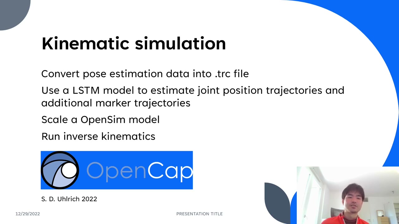
The four steps, adapted from OpenCap. Credit: S. D. Uhlrich (2022), as shown in the video.

This part is inspired by and adapted from OpenCap — an open-source project that captures motion with two iOS devices, runs OpenPose, reconstructs 3D, and then performs kinematic and kinetic simulation. Because its pipeline is open-source Python, and because we already have our own 3D data from Part 3, we can borrow OpenCap’s functions and jump straight into the simulation. Four steps:

Convert the 3D pose data into a .trc file
Augment markers with an LSTM model
Scale the OpenSim model
Run inverse kinematics

1. Convert the 3D data into a .trc file

OpenSim reads marker trajectories from a .trc file: a few header rows, then, for every frame, the x/y/z of each marker along with a frame number and time. So the first job is turning our reconstructed 3D keypoints into that format. (Recall from Part 3 that the raw keypoints are cleaned first — fill missing values by linear interpolation, then smooth with residual analysis.)

OpenCap provides a helper (writeTRCfrom3DKeypoints) that takes the 3D data, an output path, the frame rate, and optional rotation angles (a dictionary — only needed if your data is rotated; here the rotation was already fixed, so we pass none) and writes the .trc.

An honest note from the video: the reconstructed squat looks slightly tilted — likely from imperfect camera calibration or OpenPose accuracy — but the movement is clearly there, so the tutorial proceeds with it.

2. Marker augmentation with an LSTM model

OpenPose output has two limitations for biomechanics: (1) it detects each frame independently, with no link between frames, so smooth motion is hard to recover; and (2) it gives only 25 body keypoints — not enough to compute rotations at the shoulder or hip.

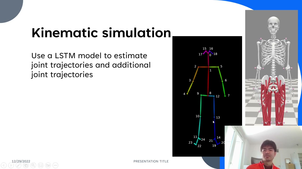
OpenPose 25-keypoint skeleton next to a musculoskeletal model with additional anatomical markers — The LSTM augments OpenPose’s 25 keypoints into a fuller anatomical marker set.

OpenCap solves both with an LSTM model trained on paired data: an optical-motion-capture marker set and the corresponding OpenPose 3D output. Because an LSTM works over a time sequence, it recovers smooth motion; and it augments extra anatomical markers (for example around the elbow and several on the hip, plus points like C7 and the ASIS/PSIS) that OpenPose never produces. Those extra markers are what make pelvis rotation, arm rotation, and flexion/extension computable.

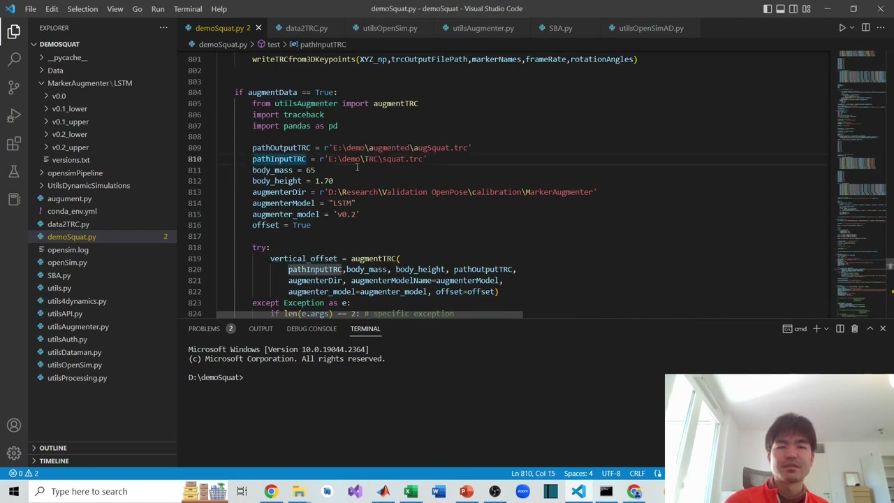
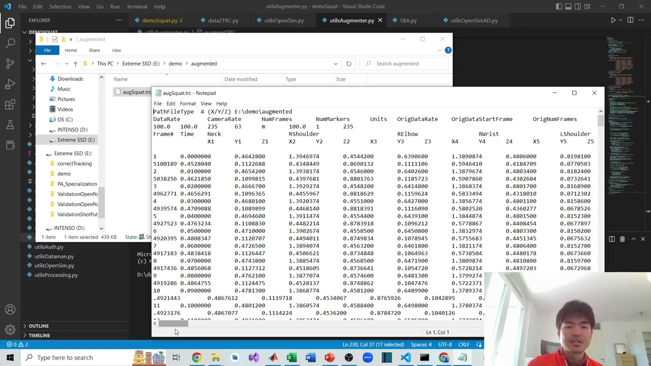
Python: writeTRCfrom3DKeypoints and augmentTRC called with body mass, body height and the LSTM model — Writing the .trc, then calling augmentTRC with body mass, body height, and the LSTM model (v0.2).

In code you call augmentTRC with the input .trc, your body mass and height, and a path to the augmenter model (several versions exist; the default is v0.2). Internally it normalizes the data, runs the LSTM, denormalizes, and writes a new augmented .trc. Opened in a text editor, that file now contains the original joints plus the estimated anatomical markers.

The augmented .trc file open in a text editor, showing header rows and X/Y/Z columns per marker — The augmented .trc: header rows, then X/Y/Z per marker (Neck, RShoulder, RElbow, RWrist, LShoulder, …).

3. Scale the OpenSim model

Next, scale a generic OpenSim musculoskeletal model to the subject using body mass, height, and a static pose. First install OpenSim (from the OpenSim website) and its Python package into a conda environment. The scaling setup XML files and the base model both come from the OpenCap repository. You pass the tracking data, the model, body mass and height, and a time range that contains the static pose, and the function writes out a scaled model.

Another candid note: the ideal static pose is a clean standing pose (see OpenCap’s documentation). The author forgot to record one, so he used the first ~1 second of standing before the squat — good enough to proceed, but not ideal, which shows up later.

4. Run inverse kinematics

Finally, run inverse kinematics: give OpenSim the scaled model and the augmented .trc, and it solves for the joint angles that best fit the markers, saving them to a .mot motion file. You can open that model and motion in the OpenSim GUI and play it back.

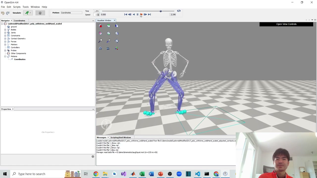
OpenSim GUI showing the scaled musculoskeletal model performing the reconstructed squat — The end result: the scaled OpenSim model performing the reconstructed squat, driven by the .mot file.

The squat is recognizable, though a bit off — the right side sinks slightly. The author attributes this to the imperfect static pose and the imperfect reconstructed data, and is upfront about how to improve it: better OpenPose data, a cleaner 3D reconstruction, and a proper static pose.

Coming next

With joint kinematics in hand, the final part goes to kinetic simulation — estimating forces, ground reaction forces, and muscle activations. Subscribe on YouTube so you don’t miss it.

About the author

Takashi Fukushima — research & development across Sports & Exercise Science, Human Pose Estimation, Computer Vision, and XR.

YouTube (subscribe): Takashi Fukushima｜Sports Science & Pose Estimation
Research (ORCID): orcid.org/0000-0002-7318-3384
Website: takashifukushima.com
Contact: Get in touch